How To Create Confidence Interval In R

Range of possible values for an unknown parameter

In statistics, a confidence interval (CI) is a range of plausible values for an unknown parameter, rather than a single estimate (for example, a population mean). The interval has an associated confidence level. A 95% confidence level is most common, but other levels, such as 90% or 99%, are sometimes used.^[1] The confidence level represents the long-run frequency of confidence intervals that contain the true value of the unknown population parameter. In other words, 95% of confidence intervals computed at the 95% confidence level contain the parameter, and likewise for other confidence levels.^[2]

The factors affecting the width of the CI include the desired confidence level, the sample size and the variability in the sample.^[3] A larger sample will tend to produce a better estimate of the population parameter, when all other factors are equal. A higher confidence level will tend to produce a broader confidence interval.^[4]

Definition [edit]

Let X be a random sample from a probability distribution with statistical parameter θ, which is a quantity to be estimated, and φ, representing quantities that are not of immediate interest. A confidence interval for the parameter θ, with confidence level or confidence coefficient γ, is an interval with random endpoints (u(X),v(X)), determined by the pair of random variables u(X) and v(X), with the property:

${\displaystyle {\Pr }_{\theta ,\varphi }(u(X)<\theta <v(X))=\gamma {\text{ for all }}(\theta ,\varphi ).}$

The quantities φ in which there is no immediate interest are called nuisance parameters, as statistical theory still needs to find some way to deal with them. The number γ, with typical values close to but not greater than 1, is sometimes given in the form 1 −α (or as a percentage 100%·(1 −α)), where α is a small non-negative number, close to 0.

Here Pr _θ,φ indicates the probability distribution of X characterised by (θ,φ). An important part of this specification is that the random interval (u(X),v(X)) covers the unknown value θ with a high probability no matter what the true value of θ actually is.

Note that here Pr _θ,φ need not refer to an explicitly given parameterized family of distributions, although it often does. Just as the random variable X notionally corresponds to other possible realizations of x from the same population or from the same version of reality, the parameters (θ,φ) indicate that we need to consider other versions of reality in which the distribution of X might have different characteristics.

In a specific situation, when x is the outcome of the sample X, the interval (u(x),v(x)) is also referred to as a confidence interval for θ. Note that it is no longer possible to say that the (observed) interval (u(x),v(x)) has probability γ to contain the parameter θ. This observed interval is just one realization of all possible intervals for which the probability statement holds.

Approximate confidence intervals [edit]

In many applications, confidence intervals that have exactly the required confidence level are hard to construct, but approximate intervals can be computed. The rule for constructing the interval may be accepted as providing a confidence interval at level ${\displaystyle \gamma }$ if

${\displaystyle {\Pr }_{\theta ,\varphi }(u(X)<\theta <v(X))\approx \gamma {\text{ for all }}(\theta ,\varphi )}$

to an acceptable level of approximation. Alternatively, some authors^[5] simply require that

${\displaystyle {\Pr }_{\theta ,\varphi }(u(X)<\theta <v(X))\geq \gamma {\text{ for all }}(\theta ,\varphi )}$

which is useful if the probabilities are only partially identified or imprecise, and also when dealing with discrete distributions. Confidence limits of form

${\displaystyle {\Pr }_{\theta ,\varphi }(u(X)<\theta )\geq \gamma }$ and ${\displaystyle {\Pr }_{\theta ,\varphi }(\theta <v(X))\geq \gamma }$

are called conservative;^[6] accordingly, one speaks of conservative confidence intervals and, in general, regions.

Desirable properties [edit]

When applying standard statistical procedures, there will often be standard ways of constructing confidence intervals. These will have been devised so as to meet certain desirable properties, which will hold given that the assumptions on which the procedure rely are true. These desirable properties may be described as: validity, optimality, and invariance. Of these "validity" is most important, followed closely by "optimality". "Invariance" may be considered as a property of the method of derivation of a confidence interval rather than of the rule for constructing the interval. In non-standard applications, the same desirable properties would be sought.

• Validity. This means that the nominal coverage probability (confidence level) of the confidence interval should hold, either exactly or to a good approximation.
• Optimality. This means that the rule for constructing the confidence interval should make as much use of the information in the data-set as possible. Recall that one could throw away half of a dataset and still be able to derive a valid confidence interval. One way of assessing optimality is by the length of the interval so that a rule for constructing a confidence interval is judged better than another if it leads to intervals whose lengths are typically shorter.
• Invariance. In many applications, the quantity being estimated might not be tightly defined as such. For example, a survey might result in an estimate of the median income in a population, but it might equally be considered as providing an estimate of the logarithm of the median income, given that this is a common scale for presenting graphical results. It would be desirable that the method used for constructing a confidence interval for the median income would give equivalent results when applied to constructing a confidence interval for the logarithm of the median income: specifically the values at the ends of the latter interval would be the logarithms of the values at the ends of former interval.

Methods of derivation [edit]

For non-standard applications, there are several routes that might be taken to derive a rule for the construction of confidence intervals. Established rules for standard procedures might be justified or explained via several of these routes. Typically a rule for constructing confidence intervals is closely tied to a particular way of finding a point estimate of the quantity being considered.

Summary statistics

This is closely related to the method of moments for estimation. A simple example arises where the quantity to be estimated is the mean, in which case a natural estimate is the sample mean. The usual arguments indicate that the sample variance can be used to estimate the variance of the sample mean. A confidence interval for the true mean can be constructed centered on the sample mean with a width which is a multiple of the square root of the sample variance.

Likelihood theory

Where estimates are constructed using the maximum likelihood principle, the theory for this provides two ways of constructing confidence intervals or confidence regions for the estimates. One way is by using Wilks's theorem to find all the possible values of ${\displaystyle \theta }$ that fulfill the following restriction:^[7]

$${\displaystyle \ln(L(\theta ))\geq \ln(L({\hat {\theta }}))-{\frac {1}{2}}\chi _{1,1-\alpha }^{2}}$$

Estimating equations

The estimation approach here can be considered as both a generalization of the method of moments and a generalization of the maximum likelihood approach. There are corresponding generalizations of the results of maximum likelihood theory that allow confidence intervals to be constructed based on estimates derived from estimating equations.^{[ clarification needed ]}

Hypothesis testing

If significance tests are available for general values of a parameter, then confidence intervals/regions can be constructed by including in the 100p% confidence region all those points for which the significance test of the null hypothesis that the true value is the given value is not rejected at a significance level of (1 −p).^[8]

Bootstrapping

In situations where the distributional assumptions for that above methods are uncertain or violated, resampling methods allow construction of confidence intervals or prediction intervals. The observed data distribution and the internal correlations are used as the surrogate for the correlations in the wider population.

Central limit theorem

The central limit theorem is a refinement of the law of large numbers. For a large number of independent endemically distributed random variables ${\displaystyle X_{1},...,X_{n},}$ with finite variance, the average ${\displaystyle {\bar {X_{n}}}}$ approximately has a normal distribution, no matter what the distribution of the ${\displaystyle X_{i}}$ is.^[9]

Example [edit]

Suppose {X ₁, …,X _n } is an independent sample from a normally distributed population with unknown (parameters) mean μ and variance σ². Let

${\displaystyle {\bar {X}}=(X_{1}+\cdots +X_{n})/n\,,}$

${\displaystyle S^{2}={\frac {1}{n-1}}\sum _{i=1}^{n}(X_{i}-{\bar {X}}\,)^{2}.}$

Where X is the sample mean, and S² is the sample variance. Then

${\displaystyle T={\frac {{\bar {X}}-\mu }{S/{\sqrt {n}}}}}$

has a Student's t distribution with n − 1 degrees of freedom.^[10] Note that the distribution of T does not depend on the values of the unobservable parameters μ and σ ²; i.e., it is a pivotal quantity. Suppose we wanted to calculate a 95% confidence interval forμ. Then, denoting c as the 97.5th percentile of this distribution,

${\displaystyle \Pr(-c\leq T\leq c)=0.95}$

Note that "97.5th" and "0.95" are correct in the preceding expressions. There is a 2.5% chance that ${\displaystyle T}$ will be less than ${\displaystyle -c}$ and a 2.5% chance that it will be larger than ${\displaystyle +c}$ . Thus, the probability that ${\displaystyle T}$ will be between ${\displaystyle -c}$ and ${\displaystyle +c}$ is 95%.

Consequently,

${\displaystyle \Pr \left({\bar {X}}-{\frac {cS}{\sqrt {n}}}\leq \mu \leq {\bar {X}}+{\frac {cS}{\sqrt {n}}}\right)=0.95\,}$

and we have a theoretical (stochastic) 95% confidence interval forμ.

After observing the sample we find values x for X and s for S, from which we compute the confidence interval

${\displaystyle \left[{\bar {x}}-{\frac {cs}{\sqrt {n}}},{\bar {x}}+{\frac {cs}{\sqrt {n}}}\right],}$

an interval with fixed numbers as endpoints, of which we can no longer say there is a certain probability it contains the parameterμ; either μ is in this interval or isn't.

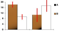
In this bar chart, the top ends of the brown bars indicate observed means and the red line segments ("error bars") represent the confidence intervals around them. Although the error bars are shown as symmetric around the means, that is not always the case. In most graphs, the error bars do not represent confidence intervals (e.g., they often represent standard errors or standard deviations)

Interpretation [edit]

Various interpretations of a confidence interval can be given (taking the 90% confidence interval as an example in the following).

• The confidence interval can be expressed in terms of samples (or repeated samples): "Were this procedure to be repeated on numerous samples, the fraction of calculated confidence intervals (which would differ for each sample) that encompass the true population parameter would tend toward 90%." ^[11]
• The confidence interval can be expressed in terms of a single sample: "There is a 90% probability that the calculated confidence interval from some future experiment encompasses the true value of the population parameter." This is a probability statement about the confidence interval, not the population parameter. This considers the probability associated with a confidence interval from a pre-experiment point of view, in the same context in which arguments for the random allocation of treatments to study items are made. Here the experimenter sets out the way in which they intend to calculate a confidence interval and to know, before they do the actual experiment, that the interval they will end up calculating has a particular chance of covering the true but unknown value.^[12] This is very similar to the "repeated sample" interpretation above, except that it avoids relying on considering hypothetical repeats of a sampling procedure that may not be repeatable in any meaningful sense. See Neyman construction.
• The explanation of a confidence interval can amount to something like: "The confidence interval represents values for the population parameter for which the difference between the parameter and the observed estimate is not statistically significant at the 10% level".^[13] This interpretation is common in scientific articles that use confidence intervals to validate their experiments, although overreliance on confidence intervals can cause problems as well.

In each of the above, the following applies: If the true value of the parameter lies outside the 90% confidence interval, then a sampling event has occurred (namely, obtaining a point estimate of the parameter at least this far from the true parameter value) which had a probability of 10% (or less) of happening by chance.

Misunderstandings [edit]

See also: § Counterexamples

Confidence intervals and levels are frequently misunderstood, and published studies have shown that even professional scientists often misinterpret them.^{[14] [15] [16] [17] [18] [19]}

• A 95% confidence level does not mean that for a given realized interval there is a 95% probability that the population parameter lies within the interval (i.e., a 95% probability that the interval covers the population parameter).^[20] According to the strict frequentist interpretation, once an interval is calculated, this interval either covers the parameter value or it does not; it is no longer a matter of probability. The 95% probability relates to the reliability of the estimation procedure, not to a specific calculated interval.^[21] Neyman himself (the original proponent of confidence intervals) made this point in his original paper:^[12]

  "It will be noticed that in the above description, the probability statements refer to the problems of estimation with which the statistician will be concerned in the future. In fact, I have repeatedly stated that the frequency of correct results will tend to α. Consider now the case when a sample is already drawn, and the calculations have given [particular limits]. Can we say that in this particular case the probability of the true value [falling between these limits] is equal to α? The answer is obviously in the negative. The parameter is an unknown constant, and no probability statement concerning its value may be made..."

Deborah Mayo expands on this further as follows:^[22]

"It must be stressed, however, that having seen the value [of the data], Neyman–Pearson theory never permits one to conclude that the specific confidence interval formed covers the true value of 0 with either (1 −α)100% probability or (1 −α)100% degree of confidence. Seidenfeld's remark seems rooted in a (not uncommon) desire for Neyman–Pearson confidence intervals to provide something which they cannot legitimately provide; namely, a measure of the degree of probability, belief, or support that an unknown parameter value lies in a specific interval. Following Savage (1962), the probability that a parameter lies in a specific interval may be referred to as a measure of final precision. While a measure of final precision may seem desirable, and while confidence levels are often (wrongly) interpreted as providing such a measure, no such interpretation is warranted. Admittedly, such a misinterpretation is encouraged by the word 'confidence'."

• A 95% confidence level does not mean that 95% of the sample data lie within the confidence interval.
• A confidence interval is not a definitive range of plausible values for the sample parameter, though it may be understood as an estimate of plausible values for the population parameter.
• A particular confidence level of 95% calculated from an experiment does not mean that there is a 95% probability of a sample parameter from a repeat of the experiment falling within this interval.^[18]

History [edit]

Confidence intervals were introduced to statistics by Jerzy Neyman in a paper published in 1937.^[23] However, it took quite a while for confidence intervals to be accurately and routinely used.

In the earliest modern controlled clinical trial of a medical treatment for acute stroke, published by Dyken and White in 1959, the investigators were unable to reject the null hypothesis of no effect of cortisol on stroke. Nonetheless, they concluded that their trial "clearly indicated no possible advantage of treatment with cortisone". Dyken and White did not calculate confidence intervals, which were rare at that time in medicine. When Peter Sandercock reevaluated the data in 2015, he found that the 95% confidence interval stretched from a 12% reduction in risk to a 140% increase in risk. Therefore, the authors' statement was not supported by their experiment. Sandercock concluded that, especially in the medical sciences, where datasets can be small, confidence intervals are better than hypothesis tests for quantifying uncertainty around the size and direction of an effect.^[24]

It wasn't until the 1980s that journals required confidence intervals and p-values to be reported in papers. By 1992, imprecise estimates were still common, even for large trials. This prevented a clear decision regarding the null hypothesis. For example, a study of medical therapies for acute stroke came to the conclusion that the stroke treatments could reduce mortality or increase it by 10%–20%. Strict admittance to the study introduced unforeseen error, further increasing uncertainty in the conclusion. Studies persisted, and it wasn't until 1997 that a trial with a massive sample pool and acceptable confidence interval was able to provide a definitive answer: cortisol therapy does not reduce the risk of acute stroke.^[24]

[edit]

Confidence region [edit]

Confidence regions generalize the confidence interval concept to deal with multiple quantities. Such regions can indicate not only the extent of likely sampling errors but can also reveal whether (for example) it is the case that if the estimate for one quantity is unreliable, then the other is also likely to be unreliable.

Confidence band [edit]

A confidence band is used in statistical analysis to represent the uncertainty in an estimate of a curve or function based on limited or noisy data. Similarly, a prediction band is used to represent the uncertainty about the value of a new data point on the curve, but subject to noise. Confidence and prediction bands are often used as part of the graphical presentation of results of a regression analysis.

Confidence bands are closely related to confidence intervals, which represent the uncertainty in an estimate of a single numerical value. "As confidence intervals, by construction, only refer to a single point, they are narrower (at this point) than a confidence band which is supposed to hold simultaneously at many points."^[25]

Prediction interval [edit]

A prediction interval for a random variable is defined similarly to a confidence interval for a statistical parameter. Consider an additional random variable Y which may or may not be statistically dependent on the random sample X. Then (u(X),v(X)) provides a prediction interval for the as-yet-to-be observed value y of Y if

${\displaystyle {\Pr }_{\theta ,\varphi }(u(X)<Y<v(X))=\gamma {\text{ for all }}(\theta ,\varphi ).\,}$

Here Pr _θ,φ indicates the joint probability distribution of the random variables (X,Y), where this distribution depends on the statistical parameters (θ,φ).

Credible interval [edit]

A Bayesian interval estimate is called a credible interval. Using much of the same notation as above, the definition of a credible interval for the unknown true value of θ is, for a given γ,^[26]

${\displaystyle \Pr(u(x)<\Theta <v(x)\mid X=x)=\gamma .}$

Here Θ is used to emphasize that the unknown value of θ is being treated as a random variable. The definitions of the two types of intervals may be compared as follows.

• The definition of a confidence interval involves probabilities calculated from the distribution of X for a given (θ,φ) (or conditional on these values) and the condition needs to hold for all values of (θ,φ).
• The definition of a credible interval involves probabilities calculated from the distribution of Θ conditional on the observed values of X =x and marginalised (or averaged) over the values of Φ, where this last quantity is the random variable corresponding to the uncertainty about the nuisance parameters inφ.

Note that the treatment of the nuisance parameters above is often omitted from discussions comparing confidence and credible intervals but it is markedly different between the two cases.

In some cases, a confidence interval and credible interval computed for a given parameter using a given dataset are identical. But in other cases, the two can be very different, particularly if informative prior information is included in the Bayesian analysis.

There is disagreement about which of these methods produces the most useful results: the mathematics of the computations are rarely in question–confidence intervals being based on sampling distributions, credible intervals being based on Bayes' theorem–but the application of these methods, the utility and interpretation of the produced statistics, is debated.^[27]

Counterexamples [edit]

Since confidence interval theory was proposed, a number of counter-examples to the theory have been developed to show how the interpretation of confidence intervals can be problematic, at least if one interprets them naïvely.

Confidence procedure for uniform location [edit]

Welch^[28] presented an example which clearly shows the difference between the theory of confidence intervals and other theories of interval estimation (including Fisher's fiducial intervals and objective Bayesian intervals). Robinson^[29] called this example "[p]ossibly the best known counterexample for Neyman's version of confidence interval theory." To Welch, it showed the superiority of confidence interval theory; to critics of the theory, it shows a deficiency. Here we present a simplified version.

Suppose that ${\displaystyle X_{1},X_{2}}$ are independent observations from a Uniform(θ − 1/2, θ + 1/2) distribution. Then the optimal 50% confidence procedure^[30] is

${\displaystyle {\bar {X}}\pm {\begin{cases}{\dfrac {|X_{1}-X_{2}|}{2}}&{\text{if }}|X_{1}-X_{2}|<1/2\\[8pt]{\dfrac {1-|X_{1}-X_{2}|}{2}}&{\text{if }}|X_{1}-X_{2}|\geq 1/2.\end{cases}}}$

A fiducial or objective Bayesian argument can be used to derive the interval estimate

${\displaystyle {\bar {X}}\pm {\frac {1-|X_{1}-X_{2}|}{4}},}$

which is also a 50% confidence procedure. Welch showed that the first confidence procedure dominates the second, according to desiderata from confidence interval theory; for every ${\displaystyle \theta _{1}\neq \theta }$ , the probability that the first procedure contains ${\displaystyle \theta _{1}}$ is less than or equal to the probability that the second procedure contains ${\displaystyle \theta _{1}}$ . The average width of the intervals from the first procedure is less than that of the second. Hence, the first procedure is preferred under classical confidence interval theory.

However, when ${\displaystyle |X_{1}-X_{2}|\geq 1/2}$ , intervals from the first procedure are guaranteed to contain the true value ${\displaystyle \theta }$ : Therefore, the nominal 50% confidence coefficient is unrelated to the uncertainty we should have that a specific interval contains the true value. The second procedure does not have this property.

Moreover, when the first procedure generates a very short interval, this indicates that ${\displaystyle X_{1},X_{2}}$ are very close together and hence only offer the information in a single data point. Yet the first interval will exclude almost all reasonable values of the parameter due to its short width. The second procedure does not have this property.

The two counter-intuitive properties of the first procedure—100% coverage when ${\displaystyle X_{1},X_{2}}$ are far apart and almost 0% coverage when ${\displaystyle X_{1},X_{2}}$ are close together—balance out to yield 50% coverage on average. However, despite the first procedure being optimal, its intervals offer neither an assessment of the precision of the estimate nor an assessment of the uncertainty one should have that the interval contains the true value.

This counter-example is used to argue against naïve interpretations of confidence intervals. If a confidence procedure is asserted to have properties beyond that of the nominal coverage (such as relation to precision, or a relationship with Bayesian inference), those properties must be proved; they do not follow from the fact that a procedure is a confidence procedure.

Confidence procedure for ω ² [edit]

Steiger^[31] suggested a number of confidence procedures for common effect size measures in ANOVA. Morey et al.^[20] point out that several of these confidence procedures, including the one for ω ², have the property that as the F statistic becomes increasingly small—indicating misfit with all possible values of ω ²—the confidence interval shrinks and can even contain only the single value ω ² = 0; that is, the CI is infinitesimally narrow (this occurs when ${\displaystyle p\geq 1-\alpha /2}$ for a ${\displaystyle 100(1-\alpha )\%}$ CI).

This behavior is consistent with the relationship between the confidence procedure and significance testing: as F becomes so small that the group means are much closer together than we would expect by chance, a significance test might indicate rejection for most or all values of ω ². Hence the interval will be very narrow or even empty (or, by a convention suggested by Steiger, containing only 0). However, this does not indicate that the estimate of ω ² is very precise. In a sense, it indicates the opposite: that the trustworthiness of the results themselves may be in doubt. This is contrary to the common interpretation of confidence intervals that they reveal the precision of the estimate.

See also [edit]

• Cumulative distribution function-based nonparametric confidence interval
• CLs upper limits (particle physics)
• Confidence distribution
• Credence (statistics)
• Error bar
• Estimation statistics
• p-value
• Robust confidence intervals
• Confidence region
• Credible interval
• Pseudoreplication

Confidence interval for specific distributions [edit]

• Confidence interval for binomial distribution
• Confidence interval for exponent of the power law distribution
• Confidence interval for mean of the exponential distribution
• Confidence interval for mean of the Poisson distribution
• Confidence intervals for mean and variance of the normal distribution

References [edit]

1. ^ Zar, Jerrold H. (199). Biostatistical Analysis (4th ed.). Upper Saddle River, N.J.: Prentice Hall. pp. 43–45. ISBN978-0130815422. OCLC 39498633.
2. ^ Illowsky, Barbara. Introductory statistics. Dean, Susan L., 1945-, Illowsky, Barbara., OpenStax College. Houston, Texas. ISBN978-1-947172-05-0. OCLC 899241574.
3. ^ Hazra, Avijit (October 2017). "Using the confidence interval confidently". Journal of Thoracic Disease. 9 (10): 4125–4130. doi:10.21037/jtd.2017.09.14. ISSN 2072-1439. PMC5723800. PMID 29268424.
4. ^ Khare, Vikas; Nema, Savita; Baredar, Prashant (2020). Ocean Energy Modeling and Simulation with Big Data Computational Intelligence for System Optimization and Grid Integration. ISBN978-0-12-818905-4. OCLC 1153294021.
5. ^ George G. Roussas (1997) A Course in Mathematical Statistics, 2nd Edition, Academic Press, p397
6. ^ Cox D.R., Hinkley D.V. (1974) Theoretical Statistics, Chapman & Hall, p. 210
7. ^ Abramovich, Felix, and Ya'acov Ritov. Statistical Theory: A Concise Introduction. CRC Press, 2013. Pages 121–122
8. ^ Cox D.R., Hinkley D.V. (1974) Theoretical Statistics, Chapman & Hall, Section 7.2(iii)
9. ^ A modern introduction to probability and statistics : understanding why and how. Michel Dekking. London: Springer. 2005. ISBN978-1-85233-896-1. OCLC 262680588. CS1 maint: others (link)
10. ^ Rees. D.G. (2001) Essential Statistics, 4th Edition, Chapman and Hall/CRC. ISBN 1-58488-007-4 (Section 9.5)
11. ^ Cox D.R., Hinkley D.V. (1974) Theoretical Statistics, Chapman & Hall, p49, p209
12. ^ ^{a b} Neyman, J. (1937). "Outline of a Theory of Statistical Estimation Based on the Classical Theory of Probability". Philosophical Transactions of the Royal Society A. 236 (767): 333–380. Bibcode:1937RSPTA.236..333N. doi:10.1098/rsta.1937.0005. JSTOR 91337.
13. ^ Cox D.R., Hinkley D.V. (1974) Theoretical Statistics, Chapman & Hall, pp 214, 225, 233
14. ^ [1]
15. ^ "Archived copy" (PDF). Archived from the original (PDF) on 2016-03-04. Retrieved 2014-09-16 . CS1 maint: archived copy as title (link)
16. ^ Hoekstra, R., R. D. Morey, J. N. Rouder, and E-J. Wagenmakers, 2014. Robust misinterpretation of confidence intervals. Psychonomic Bulletin Review, in press. [2]
17. ^ Scientists' grasp of confidence intervals doesn't inspire confidence, Science News, July 3, 2014
18. ^ ^{a b} Greenland, Sander; Senn, Stephen J.; Rothman, Kenneth J.; Carlin, John B.; Poole, Charles; Goodman, Steven N.; Altman, Douglas G. (April 2016). "Statistical tests, P values, confidence intervals, and power: a guide to misinterpretations". European Journal of Epidemiology. 31 (4): 337–350. doi:10.1007/s10654-016-0149-3. ISSN 0393-2990. PMC4877414. PMID 27209009.
19. ^ Helske, Jouni; Helske, Satu; Cooper, Matthew; Ynnerman, Anders; Besancon, Lonni (2021-08-01). "Can Visualization Alleviate Dichotomous Thinking? Effects of Visual Representations on the Cliff Effect". IEEE Transactions on Visualization and Computer Graphics. Institute of Electrical and Electronics Engineers (IEEE). 27 (8): 3397–3409. doi:10.1109/tvcg.2021.3073466. ISSN 1077-2626.
20. ^ ^{a b} Morey, R. D.; Hoekstra, R.; Rouder, J. N.; Lee, M. D.; Wagenmakers, E.-J. (2016). "The Fallacy of Placing Confidence in Confidence Intervals". Psychonomic Bulletin & Review. 23 (1): 103–123. doi:10.3758/s13423-015-0947-8. PMC4742505. PMID 26450628.
21. ^ "1.3.5.2. Confidence Limits for the Mean". nist.gov. Archived from the original on 2008-02-05. Retrieved 2014-09-16 .
22. ^ Mayo, D. G. (1981) "In defence of the Neyman–Pearson theory of confidence intervals", Philosophy of Science, 48 (2), 269–280. JSTOR 187185
23. ^ [Neyman, J., 1937. Outline of a theory of statistical estimation based on the classical theory of probability. Philosophical Transactions of the Royal Society of London. Series A, Mathematical and Physical Sciences, 236(767), pp.333-380]
24. ^ ^{a b} Sandercock, Peter A.G. (2015). "Short History of Confidence Intervals". Stroke. Ovid Technologies (Wolters Kluwer Health). 46 (8): e184-7. doi:10.1161/strokeaha.115.007750. ISSN 0039-2499. PMID 26106115.
25. ^ p.65 in W. Härdle, M. Müller, S. Sperlich, A. Werwatz (2004), Nonparametric and Semiparametric Models, Springer, ISBN 3-540-20722-8
26. ^ Bernardo JE; Smith, Adrian (2000). Bayesian theory. New York: Wiley. p. 259. ISBN978-0-471-49464-5.
27. ^ Strategic communication. davis leshan pangpang.
28. ^ Welch, B. L. (1939). "On Confidence Limits and Sufficiency, with Particular Reference to Parameters of Location". The Annals of Mathematical Statistics. 10 (1): 58–69. doi:10.1214/aoms/1177732246. JSTOR 2235987.
29. ^ Robinson, G. K. (1975). "Some Counterexamples to the Theory of Confidence Intervals". Biometrika. 62 (1): 155–161. doi:10.2307/2334498. JSTOR 2334498.
30. ^ Pratt, J. W. (1961). "Book Review: Testing Statistical Hypotheses. by E. L. Lehmann". Journal of the American Statistical Association. 56 (293): 163–167. doi:10.1080/01621459.1961.10482103. JSTOR 2282344.
31. ^ Steiger, J. H. (2004). "Beyond the F test: Effect size confidence intervals and tests of close fit in the analysis of variance and contrast analysis". Psychological Methods. 9 (2): 164–182. doi:10.1037/1082-989x.9.2.164. PMID 15137887.

Bibliography [edit]

• Fisher, R.A. (1956) Statistical Methods and Scientific Inference. Oliver and Boyd, Edinburgh. (See p. 32.)
• Freund, J.E. (1962) Mathematical Statistics Prentice Hall, Englewood Cliffs, NJ. (See pp. 227–228.)
• Hacking, I. (1965) Logic of Statistical Inference. Cambridge University Press, Cambridge. ISBN 0-521-05165-7
• Keeping, E.S. (1962) Introduction to Statistical Inference. D. Van Nostrand, Princeton, NJ.
• Kiefer, J. (1977). "Conditional Confidence Statements and Confidence Estimators (with discussion)". Journal of the American Statistical Association. 72 (360a): 789–827. doi:10.1080/01621459.1977.10479956. JSTOR 2286460.
• Mayo, D. G. (1981) "In defence of the Neyman–Pearson theory of confidence intervals", Philosophy of Science, 48 (2), 269–280. JSTOR 187185
• Neyman, J. (1937) "Outline of a Theory of Statistical Estimation Based on the Classical Theory of Probability" Philosophical Transactions of the Royal Society of London A, 236, 333–380. (Seminal work.)
• Robinson, G.K. (1975). "Some Counterexamples to the Theory of Confidence Intervals". Biometrika. 62 (1): 155–161. doi:10.1093/biomet/62.1.155. JSTOR 2334498.
• Savage, L. J. (1962), The Foundations of Statistical Inference. Methuen, London.
• Smithson, M. (2003) Confidence intervals. Quantitative Applications in the Social Sciences Series, No. 140. Belmont, CA: SAGE Publications. ISBN 978-0-7619-2499-9.

• Mehta, S. (2014) Statistics Topics ISBN 978-1-4992-7353-3
• "Confidence estimation", Encyclopedia of Mathematics, EMS Press, 2001 [1994]
• Morey, R. D.; Hoekstra, R.; Rouder, J. N.; Lee, M. D.; Wagenmakers, E.-J. (2016). "The fallacy of placing confidence in confidence intervals". Psychonomic Bulletin & Review. 23 (1): 103–123. doi:10.3758/s13423-015-0947-8. PMC4742505. PMID 26450628.

External links [edit]

• The Exploratory Software for Confidence Intervals tutorial programs that run under Excel
• Confidence interval calculators for R-Squares, Regression Coefficients, and Regression Intercepts
• Weisstein, Eric W. "Confidence Interval". MathWorld.
• CAUSEweb.org Many resources for teaching statistics including Confidence Intervals.
• An interactive introduction to Confidence Intervals
• Confidence Intervals: Confidence Level, Sample Size, and Margin of Error by Eric Schulz, the Wolfram Demonstrations Project.
• Confidence Intervals in Public Health. Straightforward description with examples and what to do about small sample sizes or rates near 0.

How To Create Confidence Interval In R

Source: https://en.wikipedia.org/wiki/Confidence_interval

Posted by: jacksonsentin2001.blogspot.com

Share this post