How To Create A Vlookup In Excel 2007

What is VLOOKUP in Excel?

The VLOOKUP function in Excel is a tool for looking up a piece of information in a table or data set and extracting some corresponding data/information. In simple terms, the VLOOKUP function says the following to Excel: "Look for this piece of information (e.g., bananas), in this data set (a table), and tell me some corresponding information about it (e.g., the price of bananas)".

Learn how to do this step by step in our Free Excel Crash Course!

VLOOKUP - someone stressed out trying to do Excel vlookup

VLOOKUP Formula

=VLOOKUP(lookup_value, table_array, col_index_num, [range_lookup])

To translate this to simple English, the formula is saying, "Look for this piece of information, in the following area, and give me some corresponding data from another column".

The VLOOKUP function uses the following arguments:

Lookup_value (required argument) – Lookup_value specifies the value that we want to look up in the first column of a table.
Table_array (required argument) – The table array is the data array that is to be searched. The VLOOKUP function searches in the left-most column of this array.
Col_index_num (required argument) – This is an integer, specifying the column number of the supplied table_array, that you want to return a value from.
Range_lookup (optional argument) – This defines what this function should return in the event that it does not find an exact match to the lookup_value. The argument can be set to TRUE or FALSE, which means:
- TRUE – Approximate match, that is, if an exact match is not found, use the closest match below the lookup_value.
- FALSE – Exact match, that is, if an exact match not found, then it will return an error.

How to use VLOOKUP in Excel

Step 1: Organize the data

The first step to effectively using the VLOOKUP function is to make sure your data is well organized and suitable for using the function.

VLOOKUP works in a left to right order, so you need to ensure that the information you want to look up is to the left of the corresponding data you want to extract.

For example:

vlookup step 1

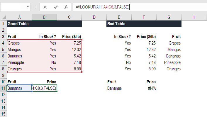
In the above VLOOKUP example, you will see that the "good table" can easily run the function to look up "Bananas" and return their price since Bananas are located in the leftmost column. In the "bad table" example you'll see there is an error message, as the columns are not in the right order.

This is one of the major drawbacks of VLOOKUP, and for this reason, it's highly recommended to use INDEX MATCH Index Match Formula Combining INDEX and MATCH functions is a more powerful lookup formula than VLOOKUP. Learn how to use INDEX MATCH in this Excel tutorial. instead of VLOOKUP.

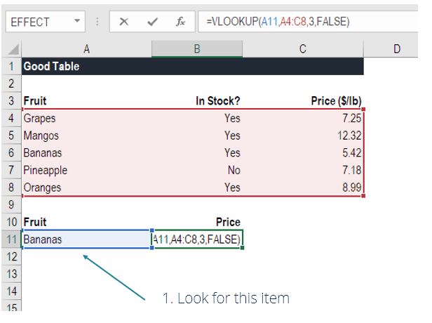
Step 2: Tell the function what to lookup

In this step, we tell Excel what to look for. We start by typing the formula "=VLOOKUP(" and then select the cell that contains the information we want to lookup. In this case, it's the cell that contains "Bananas".

vlookup step 2

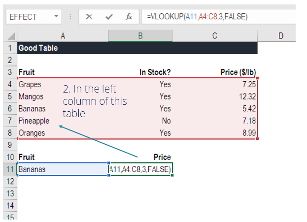
Step 3: Tell the function where to look

In this step, we select the table where the data is located, and tell Excel to search in the leftmost column for the information we selected in the previous step.

For example, in this case, we highlight the whole table from column A to column C. Excel will look for the information we told it to look up in column A.

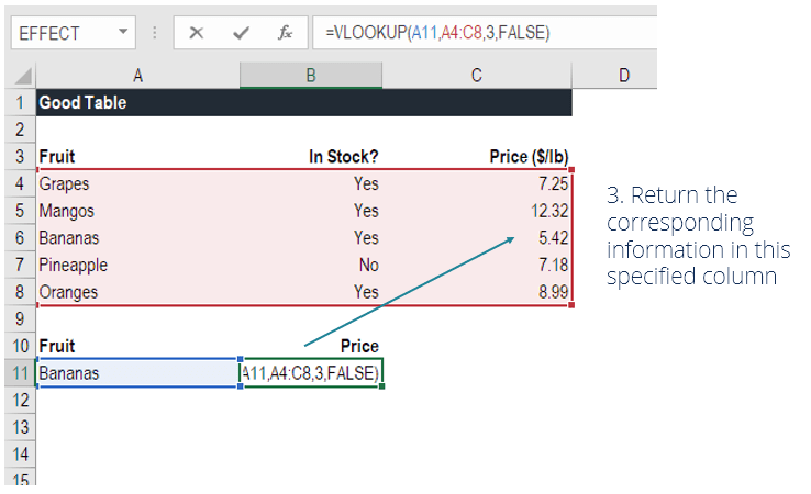
Step 4: Tell Excel what column to output the data from

In this step, we need to tell Excel which column contains the data that we want to have as an output from the VLOOKUP. To do this, Excel needs a number that corresponds to the column number in the table.

In our example, the output data is located in the 3^rd column of the table, so we enter the number "3" in the formula.

vlookup step 4

Step 5: Exact or approximate match

This final step is to tell Excel if you're looking for an exact or approximate match by entering "True" or "False" in the formula.

In our VLOOKUP example, we want an exact match ("Bananas"), so we type "FALSE" in the formula. If we instead used "TRUE" as a parameter, we would get an approximate match.

An approximate match would be useful when looking up an exact figure that might not be contained in the table, for example, if the number 2.9585. In this case, Excel will look for the number closest to 2.9585, even if that specific number is not contained in the dataset. This will help prevent errors in the VLOOKUP formula.

Learn how to do this step by step in our Free Excel Crash Course!

VLOOKUP in financial modeling and financial analysis

VLOOKUP formulas are often used in financial modeling and other types of financial analysis to make models more dynamic and incorporate multiple scenarios.

For example, imagine a financial model that included a debt schedule, where the company had three different scenarios for the interest rate: 3.0%, 4.0%, and 5.0%. A VLOOKUP could look for a scenario, low, medium or high, and output the corresponding interest rate into the financial model.

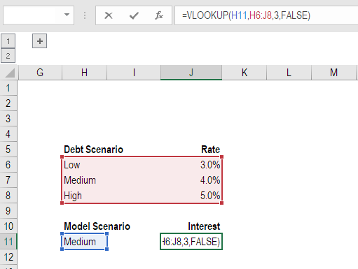
vlookup financial modeling example

As you can see in the example above, an analyst can select the scenario they want and have the corresponding interest rate flow into the model from the VLOOKUP formula.

Learn how to do this step by step in our Free Excel Crash Course!

Things to remember about the VLOOKUP Function

Here is an important list of things to remember about the Excel VLOOKUP Function:

When range_lookup is omitted, the VLOOKUP function will allow a non-exact match, but it will use an exact match if one exists.
The biggest limitation of the function is that it always looks right. It will get data from the columns to the right of the first column in the table.
If the lookup column contains duplicate values, VLOOKUP will match the first value only.
The function is not case-sensitive.
Suppose there's an existing VLOOKUP formula in a worksheet. In that scenario, formulas may break if we insert a column in the table. This is so because hard-coded column index values don't change automatically when columns are inserted or deleted.
VLOOKUP allows the use of wildcards, e.g., an asterisk (*) or a question mark (?).
Suppose in the table we are working with the function contains numbers entered as text. If we are simply retrieving numbers as text from a column in a table, it doesn't matter. But if the first column of the table contains numbers entered as text, we will get an #N/A! error if the lookup value is not also in text form.
#N/A! error – Occurs if the VLOOKUP function fails to find a match to the supplied lookup_value.
#REF! error – Occurs if either:
- The col_index_num argument is greater than the number of columns in the supplied table_array; or
- The formula attempted to reference cells that do not exist.
#VALUE! error – Occurs if either:
- The col_index_num argument is less than 1 or is not recognized as a numeric value; or
- The range_lookup argument is not recognized as one of the logical values TRUE or FALSE.

Additional resources

This has been a guide to the VLOOKUP function, how to use it, and how it can be incorporated into financial modeling in Excel.

Even though it's a great function, as mentioned above, we highly recommend using INDEX MATCH Index Match Formula Combining INDEX and MATCH functions is a more powerful lookup formula than VLOOKUP. Learn how to use INDEX MATCH in this Excel tutorial. instead, as this combination of functions can search in any direction, not just left to right. To learn more, see our guide to INDEX MATCH Index Match Formula Combining INDEX and MATCH functions is a more powerful lookup formula than VLOOKUP. Learn how to use INDEX MATCH in this Excel tutorial. .

To keep learning and developing your skills, check out these additional CFI resources:

Advanced Excel formulas list Advanced Excel Formulas Must Know These advanced Excel formulas are critical to know and will take your financial analysis skills to the next level. Download our free Excel ebook!
Excel Keyboard shortcuts Excel Shortcuts Overview Excel shortcuts are an overlooked method of increasing productivity and speed within Excel. Excel shortcuts offer the financial analyst a powerful tool. These shortcuts can perform many functions. as simple as navigation within the spreadsheet to filling in formulas or grouping data.
IF with AND functions IF Statement Between Two Numbers Download this free template for an IF statement between two numbers in Excel. In this tutorial, we show you step-by-step how to calculate IF with AND statement.
Financial modeling guide Free Financial Modeling Guide This financial modeling guide covers Excel tips and best practices on assumptions, drivers, forecasting, linking the three statements, DCF analysis, more